library(drake)
library(readr)
library(dplyr)
library(FactoMineR)A short introduction to drake
Important
The drake package has now been replaced by targets.
What is drake ?
drake is an R package which provides a way to organise and optimize your data analysis projects. For developers, it is an equivalent of GNU Make for R.
With drake, you define your project as a plan with several steps (data import, data munging, analysis, reporting…). At any time you can re-run your entire plan in a clean R environment, ensuring reproducibility. Better yet, drake looks for and takes into account dependencies between your steps, thus running only the ones needed. This can be very useful to avoid unnecessary long computations.
Here we’ll just describe a very simple project using drake. There is of course much more to look at in the drake user manual.
Project organisation
Our project will be very simple :
- load a CSV file
- cleanup data
- apply a PCA analysis
- generate an Rmarkdown report
We will organise our files like this :
data/
└── data.csv
R/
├── packages.R
├── functions_munge.R
└── plan.R
reports/
└── pca_report.Rmd
packages.R includes library calls for all required packages :
functions_munge.R will contain our data munging code, organised into functions :
data_select <- function(d) {
  d %>%
    filter(am == 1) %>%
    select(l100km, disp, hp, drat, wt, qsec)
}

data_recode <- function(d) {
  d %>%
    mutate(l100km = 379 / (1.61 * mpg))
}
Creating a plan
We are ready to define our drake plan. We will do it in the R/plan.R file by using the drake_plan function. A plan is nothing else than a named list : the list names are called targets, and identify our plan steps, and the list values are the code required to run the step. Our first step is to load our CSV file, so we could define it this way :
plan <- drake_plan(
  # Load data
  d_raw = read_csv("data/mtcars.csv")
)
What is important to understand here is that d_raw is two things at once :
- a target name, which identifies this step and allows, for example, to run it specifically
- an object name : when the step is run, the tibble returned by
read_csvwill be stored in an object namedd_raw, which will itself be cached in a specific file in a.drakefolder in your project. Thisd_rawobject will also be available in the next steps of our plan.
This would work, but it will miss a crucial functionality of drake : dependencies. With this definition, drake won’t be able to know that if the data.csv file changes, the step has to be run again. To do this, we must use the file_in function :
plan <- drake_plan(
  # Load data
  d_raw = read_csv(file_in("data/mtcars.csv"))
)
The next step to our plan is to munge our data, by applying our data_cleanup and data_recode functions. To do this, we’ll add a new target :
plan <- drake_plan(
  # Load data
  d_raw = read_csv(file_in("data/mtcars.csv")),
  # Clean data
  d = d_raw %>%
    data_recode %>%
    data_select
)
After this new step is run, a new d object will be available with our recoded ad clean data.
Next step is to run our analysis. We will do it with The PCA::FactoMineR function. This time we will call it directly, without creating a function of our own :
plan <- drake_plan(
  # Load data
  d_raw = read_csv(file_in("data/mtcars.csv")),
  # Clean data
  d = d_raw %>%
    data_recode %>%
    data_select,
  # Compute PCA
  pca = PCA(d, ncp = 4, graph = FALSE)
)
Once again, after this step is run, pca will be an available object storing our PCA results.
Running our plan
Ok, now that we defined the first steps of our plan, how can we run it ? There are several ways to do it, but the recommended one is to use the r_make() function, which will run every steps in an entire new R session, thus avoiding any possible interactions with our current global environment.
To do this, we have first to create a _drake.R file, at the root of our project, which will setup everything we need. In our case it will be :
source("R/packages.R")
source("R/functions_munge.R")
source("R/plan.R")

drake_config(
  plan,
  verbose = 2
)
This setup file will source our R scripts which will load the required packages, define our functions, and get our plan definition. Then, drake_config is used to give drake our plan object and some additional options.
Then, we can finally run our plan by running r_make() in the console :
r_make()Attachement du package : ‘dplyr’
The following objects are masked from ‘package:stats’:
filter, lag
The following objects are masked from ‘package:base’:
intersect, setdiff, setequal, union
target d_raw
Target d_raw messages:
Parsed with column specification:
cols(
mpg = col_double(),
cyl = col_double(),
disp = col_double(),
hp = col_double(),
drat = col_double(),
wt = col_double(),
qsec = col_double(),
vs = col_double(),
am = col_double(),
gear = col_double(),
carb = col_double()
)
target d
target pcar_make() will launch a new R session before running the plan. Its output shows the targets that have been built, and any message, warning or error.
If we run our plan again, the following message is shown :
All targets are already up to date.As nothing changed in our plan, nothing has to be run again.
If we make some changes, for example by changing the variables in select in our data_select function and then re-run our plan, we will get :
target d
target pcadrake is able to determine, by analysing our functions code, that our change only affects the d target and the subsequent pca target, but not d_raw. It thus runs only the affected steps.
Cache
When using r_make(), one thing can be a bit surprising : our plan has been run, all computations and analysis have been made, but our environment is unmodified : no new object has been created, d_raw, d or pca are nowhere to be seen. That’s because these objects are stored in a cache, by default files in a .drake folder in your project root.
So, what if we want to access these objects ?
drake offers several functions to interact with objects in cache.
The first is readd(), which allows to read an object from cache by giving its name :
my_d <- readd(d)The second is loadd(), which loads a cached object directly into the environment. Thus this :
loadd(pca)Is equivalent to this :
pca <- readd(pca)Finally, loadd() without arguments loads every cached objects into the environment at once (be careful if there are very large datasets or computation results) :
loadd()There are several other cache related functions, such as clean(), which invalidates all cached objects and forces their recomputations the nex time the plan is run. There are also much more about cache, such different storage formats, or garbage collection : please refer to the user manual.
Rmarkdown documents
What if we now want to add an Rmarkdown report as the last step of our plan ? Well, first we have to write the correspondig Rmd file, which we’ll put in a reports folder. Inside this file, we can access the objects created in previous plan targets by using readd or loadd. So for example one of our first chunks coud include something like1 :
library(drake)
loadd(d)
loadd(pca)
Then we have to add the step to our plan. This target will directly invoke rmarkdown::render, something like this :
plan <- drake_plan(
  ## Load data
  d_raw = read_csv(file_in("data/mtcars.csv")),
  ## Clean data
  d = d_raw %>%
    data_recode %>%
    data_select,
  ## Compute PCA
  pca = PCA(d, ncp = 4, graph = FALSE),
  ## Generate report
  pca_report = rmarkdown::render(
    input = knitr_in("reports/pca_report.Rmd"),
    output_file = "pca_reports.html"
  )
)
Note that the input file name has been wrapped into a knitr_in() call : this will both make the file tracked for changes, and analyse its code chunks to track for objects dependencies, so that the document will be regenerated if any previous objects used have changed.
Running our plan (again)
Our plan is now completely defined, and each time we run r_make(), everything from data loading to reporting will be done, only if necessary. Thanks to drake dependencies handling, this allows for minimal execution and waiting time each time we change something in our data, code or report.
Sometimes you may want to force the recomputation of a specific target, or limit the computation to this target without triggering others. This can be done with r_drake_build() :
r_drake_build(target = "pca")You can even interactivly visualize your project dependencies, and the status of each plan target with vis_drake_graph :
source("_drake.R")
config <- drake_config(plan)
vis_drake_graph(config)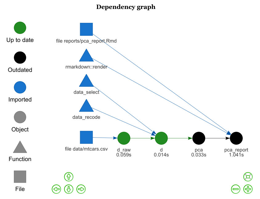
Limitations and workarounds
Step names
Obviously, two different targets can’t have the same name. This can be a bit confusing at first, when you are used to doing things like this :
d <- read_csv(file_in("data/mtcars.csv")),
d <- d %>%
    data_recode %>%
    data_select
Which cannot be translated into :
plan <- drake_plan(
  d = read_csv(file_in("data/mtcars.csv")),
  d = d %>%
    data_recode %>%
    data_select
)
So you’ll have to use different names for each step and associated object. But I think it is a good thing as, for example, it will force to describe, separate and organise different munging operations instead of having one big munging R script.
Interactivity
Another limitations is that you cannot add “interactive” functions in a plan target, such as a shiny app, or even a call to a base plot()2.
One workaround can be to create an interactive.R script somewhere with just the needed code, ready to be run if you wish to. For example, if you’d like to visualize your PCA results with explor3, you can do the following :
library(drake)
library(explor)

loadd(pca)
explor(pca)
htmlwidgets
One problem I faced during my tests was when trying to insert some htmlwidgets, such as leaflet maps, inside Rmarkdown documents. The r_make() call then fails with a cannot remove bindings from a locked environment error message.
The workaround is to wrap the render into a callr::r call, like this :
report = callr::r(
    function(...) rmarkdown::render(...),
    args = list(
      input = knitr_in("reports/in.Rmd"),
      output_file = "out.html"
    )
  )
For more details and explanations, see this issue.
Conclusion
Of course, there is much more to drake than what is presented here. This is a quite deep package with many functions from cache management to high performance computing. Furthermore, drake is quite agnostic on your code organisation, so the way code is organised in this post can really be deeply and adapted to your workflow.
Using drake adds a bit of rigidity and complexity to your project, but after playing with it a bit I think that this is vastly balanced by the advantages :
drakeforces you to organise your project as a well-defined and organised series of steps, which is easily readable and understandable from your plan object, for you or for someone else.drakeforces you to organise your code into (pure) functions and benefit from functional programming paradigm.drakefavors rmarkdown documents as analyses results, instead of separate graphs or text outputs.drakeallows and guarantees the reproducibility of your work.drakeallows efficiency and minimal execution time when something in your project changes.
For more information, you can refer to the package website and to the very complete user manual.
Notes
An alternative couls be to pass them as parameters↩︎
You can use graphical functions that return plots as an object, such as
ggplot2. The resulting plot object can then be displayed withreadd()↩︎Sorry, shameless autopromotion…↩︎